Score

See the full API for the module at Score Module.

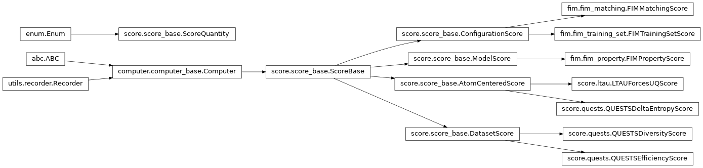
The Score class encapsulates the functionality for computing and storing “scores” of atomic environments or atomic configurations. Common examples would be UQ metrics or “importance” scores.

An AtomCenteredScore is computed for each local atomic environment (an atom and its neighbors within a cutoff). An example would be an LTAU UQ metric. ConfigurationScore is computed for an entire supercell. An example would be a FIM.

Designing a Score Module

If you are developing a new Score module, then it will be useful to understand a few key design choices that were made.

When executing a calcuation using the run() function, the arguments used for initializing a Computer, and the arguments passed to the compute() call, will be written out to temporary folders. This is done so that the module can be re-initialized and the calculation can be performed within a batch job that may not have access to the original class instance. In the case of array-like arguments, these values will be saved as .npy file. In order to support this functionality, you should make sure that your __init__() function can optionally read any array-like arguments from a file. These files will be removed by the cleanup() function once the job is completed.

LTAU Forces UQ Score

The LTAUForcesUQScore module provides ensemble-based uncertainty quantification for force predictions. This module uses distributions of force error magnitudes sampled over the course of training to estimate uncertainty for each atom. For test atoms, a nearest-neighbor search is performed in descriptor space using the FAISS library.

Key features:

• Supports building PDFs from error logs or pre-computed distributions

• Uses FAISS for efficient nearest-neighbor search in descriptor space

• Configurable binning strategies (linear or logarithmic spacing)

• Multiple index types supported (IndexFlatL2, IndexHNSWFlat, etc.)

Usage example:

ltau_score = LTAUForcesUQScore(
    train_descriptors=descriptors,  # (num_atoms, num_dimensions)
    error_pdfs=error_logs,  # (num_epochs, num_atoms)
    index_type='IndexFlatL2',
    from_error_logs=True,
    nbins=100,
)

uncertainties = ltau_score.compute_batch(
    dataset,  # list of ASE Atoms
    ScoreQuantity.UNCERTAINTY,
    descriptors_key='descriptors',
    num_nearest_neighbors=5
)

QUESTS Score Modules

The QUESTS modules provide information-theoretic measures of dataset quality using kernel density estimation. Three complementary scores are available:

QUESTSEfficiencyScore

Measures dataset efficiency as the ratio H/maxH, quantifying how little redundancy the dataset contains. Values near 1 indicate minimal oversampling.

QUESTSDiversityScore

Estimates how well the dataset covers the configuration space it spans. Higher values indicate better coverage of the accessible regions.

QUESTSDeltaEntropyScore

Computes per-atom estimates of entropy increase when adding points to a reference set. Useful for identifying configurations that would add the most information.

All QUESTS modules use Gaussian kernel density estimation with configurable bandwidth and support optional environment selection masks.

Usage examples:

# Dataset efficiency
efficiency_score = QUESTSEfficiencyScore()
efficiency = efficiency_score.compute(
    dataset=dataset,  # list of ASE Atoms
    score_quantity=ScoreQuantity.EFFICIENCY,
    descriptors_key='descriptors',
    bandwidth=0.1
)

# Per-atom delta entropy
delta_entropy_score = QUESTSDeltaEntropyScore()
delta_entropies = delta_entropy_score.compute_batch(
    dataset,  # list of ASE Atoms
    ScoreQuantity.DELTA_ENTROPY,
    reference_set=descriptors,  # (num_atoms, num_dimensions)
    bandwidth=0.1,
    descriptors_key='descriptors',
)

Fisher Information Matrix (FIM) Modules

In theory, the FIM measures the expected information that data contains about potential parameters. Assuming a Gaussian likelihood, the FIM can be calculated by taking the dot product between the Jacobian matrix with itself, where the Jacobian contains the partial derivative of the correspoding model output with respect to its parameters. This concept is further utilized in the information-matching method [1] for active learning.

There are three separate FIM modules that are needed to use the information-matching method. These modules are typically used in the following order: (1) use FIMTrainingSetScore to compute the FIM of each atomic configuration using the training quantities, e.g. configuration energy and atomic forces, (2) use FIMPropertyScore to compute the FIM of the target properties, and (3) use FIMMatchingScore to use information-matching method to compute the optimal weight for each candidate atomic configuration.

Note

FIMTrainingSetScore and FIMPropertyScore are currently only compatible with KIMPotential. Furthermore, FIMPropertyScore only supports the potentials capable of writing parameters. FIMMatchingScore only uses the FIMs computed by the other two calculations and does not require a potential.

The FIM computed using FIMTrainingSetScore or FIMPropertyScore approximates the Hessian of the potential. Specifically, each element at row \(i\), column \(j\) represents the second derivative of the potential predictions with respect to the parameters at indices \(i\) and \(j\). The mapping between parameter indices and their corresponding parameters is stored in fim_index_to_parameter attribute.

As an example consider computing the FIM for the Stillinger-Weber potential in OpenKIM, with KIM ID SW_StillingerWeber_1985_Si__MO_405512056662_006. We take derivatives only with respect to parameters \(A\) and \(B\) by specifying:

parameters_optimize={
    'A': [[15.2848479197914]],
    'B': [['default']],
    'lambda': [[0.0, 'fix']]
}

This results in a \(2 \times 2\) FIM, where:

• The (0, 0) element corresponds to the second derivative w.r.t. \(A\),

• The (0, 1) and (1, 0) elements correspond to mixed derivatives w.r.t. \(A\) and \(B\),

• The (1, 1) element corresponds to the second derivative w.r.t. \(B\).

The attribute fim_index_to_parameter outputs:

{
    0: {"parameter": "A", "extent": 0},
    1: {"parameter": "B", "extent": 0}
}

Here, the dictionary keys represent parameter indices, while the values contain the parameter name and its extent. If a parameter has multiple values (e.g., different interaction types), extent reflects this structure.

[1]

Y. Kurniawan et al., “An information-matching approach to optimal experimental design and active learning,” Nov. 05, 2024, arXiv: arXiv:2411.02740. doi: 10.48550/arXiv.2411.02740.

FIMTrainingSetScore

This module is used to compute the FIM of energy, forces, etc. of each atomic configuration. The derivative is done numerically using numdifftools Python package, which uses Richardson’s extrapolation to achieve high-accuracy derivative estimation.

As an example, suppose we want to compute the FIM for a Stillinger-Weber potential for silicon, which is stored in OpenKIM. The KIM ID for this potential is SW_StillingerWeber_1985_Si__MO_405512056662_006. Let’s compute the FIM for the atomic forces quantity only (no energy or stress), and we take the derivative with respect to the two-body energy scaling parameters (i.e., A and B).

An example code to do this calculation using FIMTrainingSetScore is given below.:

from orchestrator.computer.score.fim import FIMTrainingSetScore
from ase.io import read

# Candidate configurations as ase.Atoms objects
# candidate_configurations.xyz is just a dummy configuration file name.
list_of_atoms = read('candidate_configurations.xyz', format='extxyz', index=':')
nconfigs = len(list_of_atoms)

# Compute the FIM for each atomic configuration
myfim_training_set = FIMTrainingSetScore()
fim_training_set = myfim_training_set.compute_batch(
    list_of_atoms=list_of_atoms,
    score_quantity='SENSITIVITY',  # This value should be changed
    potential={
        'potential_type': 'KIM',
        'potential_args': {
            'kim_id': 'SW_StillingerWeber_1985_Si__MO_405512056662_006',
            'kim_api': 'kim-api-collections-management'
        }
    },
    parameters_optimize={
        'A': [[15.2848479197914]],
        'B': [['default']],
        'lambda': [[0.0, 'fix']]
    },
    # Optional - The defult is to compute the forces only
    evaluate_kwargs={
        'compute_energy': [False] * nconfigs,
        'compute_forces': [True] * nconfigs,
        'compute_stress': [False] * nconfigs
    },
    # Optional - The default is to use central difference method with step
    # size 10% of the potential parameters. This argument is passed in as
    # keyword arguments to numdifftools.Jacobian.
    derivative_kwargs={'method': 'central'}
)

# Save the results to score_results.xyz
myfim_training_set.save_results(
    compute_results=fim_training_set, list_of_configs=list_of_atoms)

Note

Energy, force, and stress have different physical units. Since FIMTrainingSetScore does not handle the weighting of these quantities internally, each configuration should be used to compute only one quantity at a time. Specifically, there should be exactly one True value among the compute_energy, compute_forces, and compute_stress keys in the evaluate_kwargs argument.

If multiple quantities need to be evaluated for the same configuration, the configuration should be duplicated, with each duplicate assigned a different quantity.

When computing the FIM using atomic forces quantity, one can pass a binary masking array, e.g., [1, 1, 1, 0, 0, 0], to include or exclude rows of the Jacobian, effectively include and exclude the prediction contribution of certain atoms in the configuration. For the specific masking array example above, it excludes the cartesian force components acting on the second atom.

Note

If there are multiple atomic configurations, one masking array should be specified for each of them. A special value is None, in which case there is no rows in the Jacobian excluded. A .npy or .txt file that contains the masking array that can be read via np.load or np.loadtxt can also be used.

FIMPropertyScore

This module is used to estimate the FIM of the target property, such as elastic constants. Since the target property calculations are typically expensive, the derivative is estimated numerically using regular finite difference method.

As an example, suppose we want to compute the FIM for the elastic constant of diamond silicon. Let’s still use the same SW potential with the same set of potential parameters. For information-matching calculation, we also need to specify a target covariance matrix for the target property. The information- matching calculation will determine a set of optimal weights for the training configurations such that the uncertainty of the target property is smaller than this target covariance. For simplicity, we can assume that the target covariance for this example is just an identity matrix.

An example code to do this calculation using FIMPropertyScore is given below.:

from orchestrator.computer.score.fim import FIMPropertyScore
import numpy as np

myfim_property = FIMPropertyScore()
fim_property = myfim_property.compute(
    list_of_target_property=[
        {
            'init_args': {
                'target_property_type': 'ElasticConstants',
                'target_property_args': {
                    'lattice_param': 5.43,
                    'lattice_type': 'diamond',
                    'deformation_mag': 0.0001,
                    'simulator_path':
                    '/PATH/TO/lmp',
                    'elements': ['Si']
                }
            },
            'calculate_property_args': {
                'workflow': {
                    'workflow_type': 'LOCAL',
                    'workflow_args': {}
                }
            }
        }
    ],
    score_quantity='SENSITIVITY',  # This value should be changed
    cov=np.eye(36),  # Target covariance matrix for the target properties
    potential={
        'potential_type': 'KIM',
        'potential_args': {
            'kim_id': 'SW_StillingerWeber_1985_Si__MO_405512056662_006',
            'kim_api': 'kim-api-collections-management'
        }
    },
    parameters_optimize={
        'A': [[15.2848479197914]],
        'B': [['default']],
        'lambda': [[0.0, 'fix']]
    },
    # Optional - Additional argument for the finite difference derivative,
    # which only includes the step size and string pointer for the method.
    derivative_kwargs={'h': 0.1, 'method': 'CD'},
)

# Save the results to score_results.json
myfim_property.save_results(compute_results=fim_property)

FIMMatchingScore

This module wraps over Python package information-matching to compute the optimal weight to assign to each candidate atomic configurations. This calculation requires the other FIM calculations first.

Continuing with the examples above, we can use the following code to compute the optimal weights for the configuration using FIMMatchingScore:

from orchestrator.computer.score.fim import FIMMatchingScore
from ase.io import read

# Load the FIMs
list_of_atoms = read('score_results.xyz', format='extxyz', index=':')
fim_property = 'score_results.json'

# information-matching calculation
myfim_matching = FIMMatchingScore()
fim_matching = myfim_matching.compute_batch(
    list_of_atoms=list_of_atoms,
    fim_property=fim_property,
    score_quantity='IMPORTANCE',  # This value should be changed
    # Optional - keyword arguments to instantiate information_matching.ConvexOpt
    convexopt_init_kwargs={'weight_upper_bound': None},
    # Optional - keyword arguments to solve convex optimization problem via
    # cvxpy
    solver_kwargs={'solver': 'SDPA', 'verbose': True},
    # Optional - tolerances for extracting non-zero weights
    weight_tolerance={'zero_tol': 1e-4, 'zero_tol_dual': 1e-4}
)

# Save the results to score_results.xyz
myfim_matching.save_results(compute_results=fim_matching, list_of_configs=list_of_atoms)
print(fim_matching)

Inheritance Graph